Our 2026 Capital Markets Assumptions (CMAs) represent the ongoing evolution of our 10 year forward looking market forecasts, which serve as the cornerstone of our Strategic Asset Allocation(SAA) framework—the bedrock of our clients’ investment programs. A disciplined, forward-looking investment process is paramount to achieving consistent and dependable outcomes, a standard we have upheld for nearly 25 years. Grounded in Modern Portfolio Theory pioneered by Nobel laureate Harry Markowitz, our methodology is designed to construct robust return expectations that align with the asset allocation models employed by sophisticated institutional investors. Rather than assessing individual assets in isolation, we take a holistic view, emphasizing their collective influence on portfolio dynamics to foster resilience and long-term stability.
Benjamin Grahm once noted, “The essence of investment management is the management of risks, not the management of returns.” This insight feels especially relevant in today’s environment. In such an environment, a disciplined approach to decision-making is essential for long-term success. At Baker Street, we are proud to serve as a trusted advisor, offering clarity and strategic insight into an increasingly complex financial landscape. Our risk-based framework has guided clients through evolving market conditions, helping them navigate uncertainty with confidence. However, our role transcends mere portfolio management; we seek to instill confidence through a steadfast investment philosophy designed to endure volatility. As Morgan Housel astutely observes in The Psychology of Money, “Controlling your time is the highest dividend money pays.” Through disciplined stewardship, we empower our clients to prioritize what truly matters, secure in the knowledge that their financial foundation is engineered to withstand the uncertainties of the market.
For more details, the expanded sections below offer a deeper dive into our methodology and process. In summary, our approach blends academic rigor with practical application to evaluate risk, return, correlation, and tax implications—forming the basis for portfolios designed to deliver optimal long-term outcomes for our clients
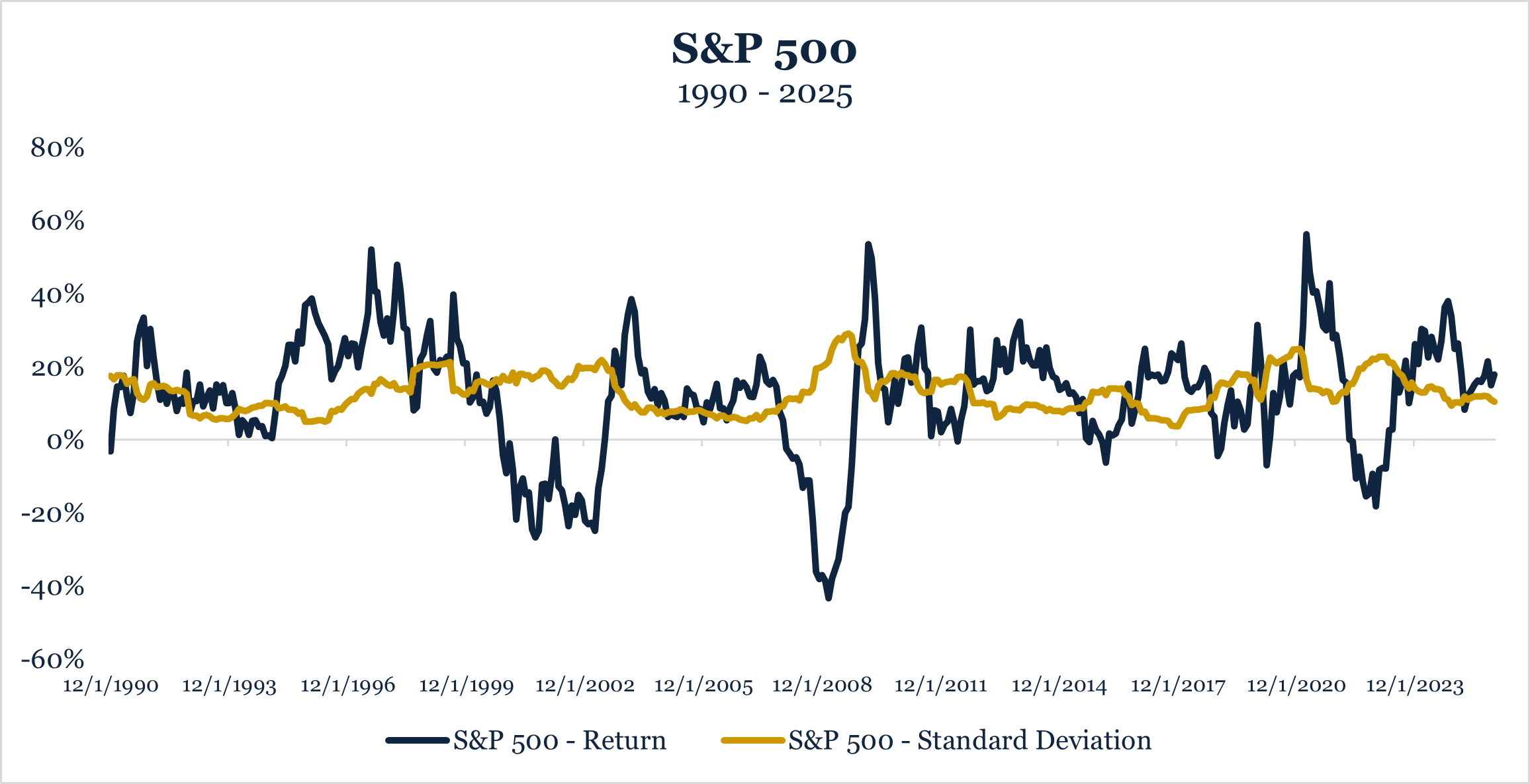
Capital Market Assumptions can be broadly classified into two categories: risk and return. Empirical evidence indicates that predicting risk is much easier than forecasting returns. To estimate risk, we employ well-established methodologies that account for the dynamic nature of markets while incorporating long-term trends. This structured approach provides a robust foundation for risk estimation. The greater challenge, however, lies in forecasting returns and integrating them effectively into our modeling. Short-term return predictions are particularly unreliable due to market volatility, whereas asset class risk—quantified by the standard deviation of returns—tends to exhibit greater stability (refer to the chart below).
Traditional return models used in asset allocation often lead to suboptimal outcomes, primarily due to an overdependence on recent historical performance, long-term expected returns, or aggregated analyst forecasts. These approaches are susceptible to both behavioral biases and empirical shortcomings, including inconsistent historical trends, excessive volatility that triggers abrupt portfolio adjustments, asset concentration risks, and internally inconsistent return projections. To mitigate these pitfalls, our approach emphasizes return forecasts that prioritize stability, cross-asset class consistency, and a comprehensive estimation process that evaluates asset classes in an integrated manner rather than in isolation. This methodology fosters a more reliable and diversified framework for return estimation.
Our process begins with the “Market Portfolio” (See step 1 below), which serves as the foundation for return assumptions when combined with our risk estimates. These return projections are designed to evolve gradually over a 10-year forecast horizon, ensuring stability and the development of a well-diversified portfolio. The following sections provide a detailed exposition of our methodology.
In Modern Portfolio Theory(MPT), the market portfolio is a theoretical construct that encompasses all investable assets, weighted by their market value. It represents the most diversified portfolio and is considered the optimal risky portfolio for investors. Since the theoretical market portfolio is not directly investable and hard to define, we create a representative portfolio by analyzing the allocations of the largest U.S. endowments—those managing over $5 billion in assets, as tracked by the National Association of College and University Business Officers(NACUBO4).
At its core, this is an institutional-grade portfolio designed to approximate the Market Portfolio, drawing upon the investment philosophies and allocations of some of the world’s most sophisticated institutional investors. These endowments include esteemed institutions such as Harvard University, Yale University, and Stanford University, among many others.
We use the average asset allocation of these $5B+ NACUBO endowments and ultimately adjusting for taxes(see Steps 4-6).
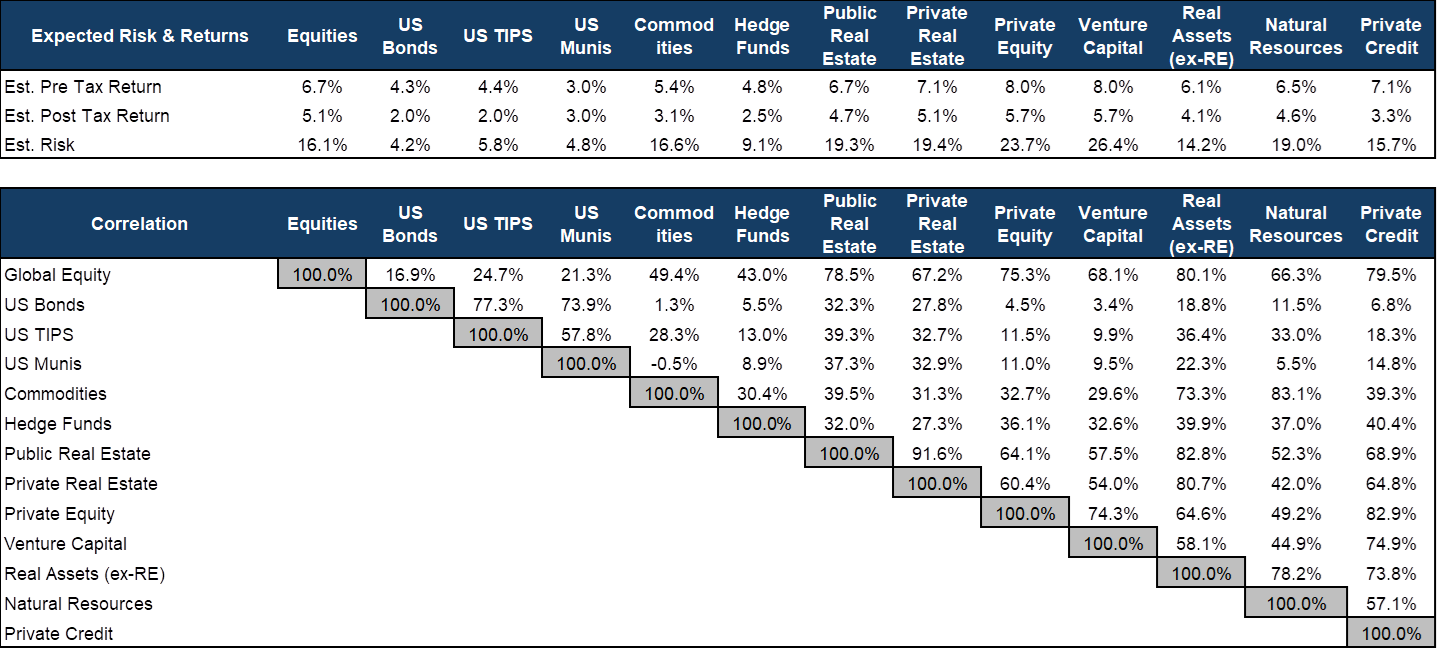
For each asset class in our model, we use a proxy to estimate risk and correlations. Typically, we select public securities that we believe most accurately represent a given asset class. For example, we use the iShares MSCI ACWI ETF as a proxy for Global Equity.
Similarly, for private asset classes, we rely on carefully chosen publicly traded proxies to develop risk and correlation assumptions. Private assets, such as Private Equity and Private Credit, are inherently challenging to assess due to their infrequent valuations and lack of standardized pricing. Traditional approaches often underestimate the true volatility and correlation of these asset classes, leading to misinformed portfolio construction. To address this, we use proxies that exhibit comparable risk-return characteristics and market behaviors. For example, we utilize the iShares Micro-Cap ETF as a proxy for Private Equity, as micro-cap public equities tend to exhibit similar risk profiles and economic sensitivities.
It is important to emphasize that in our model, these proxies are primarily used to derive risk and correlation estimates, rather than direct return projections. Our return estimation methodology, which incorporates a more comprehensive framework, is detailed in Step 4.
We recognize that periods of elevated market stress occur more frequently than a traditional normal distribution (bell curve) would suggest. To account for this, we categorize asset class’s proxy return stream into two periods: “Normal” and “Crisis.” In our2026 modeling, we assign a 22% weighting to crisis periods, emphasizing the importance of constructing portfolios that can endure market stress for long-term stability. We define a crisis period as any month where annualized equity market volatility exceeds 21% (compared to long-term averages of approximately 15%). Since 2000, 19% of months have met this criterion, meaning our current modeling conservatively gives approximately 15% more weight to the past 25 years of "crisis" periods.
In our framework, all past crisis periods are given equal weight, acknowledging the inherent uncertainty of what a future crisis may entail. For “normal” periods, we assume that recent market conditions are more indicative of future trends than those from the distant past. To reflect this, we apply a time-based weighted average, ensuring that more recent data has a slightly greater influence on our modeling than older data. This weighted average is achieved using an “exponentially decaying ”weighting with a “half-life” of 84 months, meaning the most recent month of data is weighted twice as heavily as the data from 84 months ago. In simpler terms, the weight of a month decreases by half every 84 months. The rationale behind this approach is that future “normal” market conditions are likely to reflect the recent past more closely, including factors such as market concentration, yield curve environment, investment themes, and macroeconomic conditions.
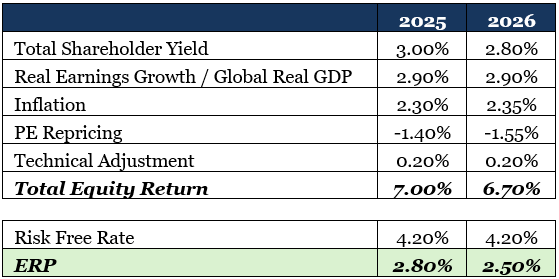
The equity risk premium (ERP)represents the difference between the expected return of equities and the risk-free rate of return. We use US Treasury yields to determine our risk-free rate assumption, which for this year’s update is 4.2%.
To calculate the equity risk premium, we apply the Grinold-Kroner model to estimate expected equity returns3.This framework suggests that future equity returns are the sum of the total shareholder return (dividend yield + buyback yield), expected inflation, the real growth rate of earnings, and changes in the Price-to-Earnings ratio.
As previously mentioned, our risk assumptions serve as the foundation for our return expectations. In alignment with the Modern Portfolio Theory framework, we apply the Capital Asset Pricing Model (CAPM) to estimate pre-tax asset class returns. CAPM establishes a relationship between expected return and risk, asserting that the expected return of a security or asset class is equal to the risk-free rate plus a risk premium. This risk premium reflects the compensation investors require forbearing additional risk relative to a risk-free asset.
In our approach, the risk premium is determined based on the asset class's risk relative to a well-diversified proxy market portfolio. Specifically, we estimate each asset class’s beta—its sensitivity to the reference market portfolio—and use this to scale the risk premium accordingly. This ensures that riskier asset classes, which exhibit higher volatility and market sensitivity, are assigned higher expected returns in accordance with CAPM principles.
Additionally, we recognize that certain asset classes, may not align perfectly with traditional CAPM assumptions due to factors such as liquidity constraints, idiosyncratic risks, portfolio concentration, and manager-specific influences. To account for these nuances, we supplement our CAPM-based return estimates with additional adjustments informed by historical risk premia, empirical studies, and forward-looking macroeconomic expectations.
The result is a structured, risk-driven approach to return estimation that maintains consistency across asset classes while incorporating market realities. Our pre-tax return estimates, derived from this methodology, can be found in the table on page 1.
For each asset class, we make assumptions about the various components of return (e.g., interest, dividends, long-term capital gains, etc.) and apply a client's effective tax rate to each of these components. Additionally, we consider the client’s Expected holding period for each asset class. This assumption acknowledges that some asset classes (e.g., Public Equity) do not incur full tax liabilities every year, allowing investors to defer taxes and let those deferrals compound over time. We believe this is a critical factor in modeling after-tax expected returns, as it enables more precise optimization of asset allocation across asset classes with different turnover rates.
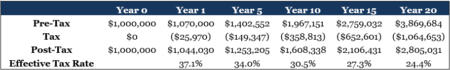
The table below illustrates the effective tax rate for a California taxpayer who defers capital gains on public equity investments for periods ranging from 1 to 20 years, assuming a pre-tax7% annual growth rate (assuming no dividends and no taxes paid until liquidation). As shown, extending the deferral period reduces the effective tax rate. For instance, an investment with a 5-year turnover incurs a 40% higher effective tax rate than one with a 20-year turnover (34.4% vs. 24.4%). This highlights the importance of considering holding periods when constructing optimal post-tax portfolios. You can see our post-tax return estimates in the table on page 1.
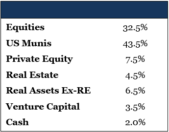
Once steps 1 through 5 are complete, we can optimize and identify allocations that we believe will generate the highest after-tax return for a given level of risk for our clients over the coming years. We also do this within the context of any portfolio-level constraints. For example, the asset allocation below shows our optimized recommendation for a highest marginal tax bracket California client with a moderate-risk portfolio (estimated 9.5% standard deviation).